Linear Transformation Properties

The Two Linearity Conditions

A function

T: V \to W

is linear if it satisfies two conditions for all

\mathbf{u}, \mathbf{v} \in V

and all scalars

c \in \mathbb{R}

:

Additivity:

T(\mathbf{u} + \mathbf{v}) = T(\mathbf{u}) + T(\mathbf{v})

Homogeneity:

T(c\mathbf{v}) = cT(\mathbf{v})

Both conditions must hold for every choice of vectors and scalars — not just for specific examples. Verifying linearity on a few particular vectors does not suffice. Disproving linearity requires only a single counterexample: one pair of vectors where additivity fails, or one scalar where homogeneity fails.

Linearity Notation

Notation

Linearity Notation

The definition of a linear map is written with one set of symbols standing for two sets of operations. Four marks decide what the equation is actually claiming.

The bracket

[T]

that turns a map into an array, the chaining rule for compositions and the reason the rightmost factor acts first are set out at matrix representation. Coordinate brackets and the script letters used for bases belong to basis, and

\dim

with its field subscript to dimension.

T(c\mathbf{u} + d\mathbf{v}) = cT(\mathbf{u}) + dT(\mathbf{v})

T of c u plus d v equals c times T of u plus d times T of v

Four operations appear here and they are not the same four. The addition and the scaling on the left are performed in

V

, before

T

is applied; the ones on the right are performed in

W

, after. One glyph is reused for both, and the equation is precisely the claim that the two structures agree.

CasesSetting

c = d = 1

leaves additivity; setting

\mathbf{v} = \mathbf{0}

leaves homogeneity. The single line is not a shorthand for the pair — it implies both, and both together imply it.

Also writtenSplit into two displayed conditions when each is being checked separately, which is the usual form in a proof and hides that one equation carries both.

Do not confuseReading the line as an identity to be simplified. It is a condition to be tested: a hypothesis about a particular

T

, true for some functions and false for most, and nothing about the symbols guarantees it.

Same glyph elsewhereThe plus sign inside

T(\cdot)

and the plus sign outside it denote different operations in different spaces throughout this page. Nothing marks the difference except position.

T(\mathbf{0}_V) = \mathbf{0}_W, \qquad T^{-1} \circ T = I_V

T of the zero of V is the zero of W; T inverse after T is the identity on V

The subscripts name which space the object belongs to. There are two zero vectors here and two identity maps, and without the labels the first equation reads as though nothing happened and the second as though one identity were being used twice.

CasesWhen

V

and

W

are the same space the subscripts are dropped and nothing is lost. They earn their place exactly when a map crosses between spaces, which is also when the statement stops being obvious.

Also writtenWritten

\mathbf{0}

and

I

unadorned in most sources, leaving the reader to supply the space from the surrounding line.

Do not confuseTaking

T(\mathbf{0}) = \mathbf{0}

for part of the definition. It is a consequence, and it works in one direction only: failing it disproves linearity outright, while passing it proves nothing —

T(x) = x|x|

sends

0

to

0

and is not linear.

T(x, y, z) = (2x - y, \; x + 3z)

T of the triple x, y, z is the pair two x minus y, x plus three z

The parentheses after

T

are doing two jobs at once. Written strictly the line would begin

T\big((x, y, z)\big)

, with the inner pair building a vector and the outer pair applying the function; one pair is dropped by convention.

T

takes a single argument, not three.

CasesOn the right the parentheses have only the tuple job — there is no function being applied there. The same glyph carries two meanings on the left and one on the right, in a single line.

Also writtenThe argument is written

T(\mathbf{v})

with a bold letter elsewhere on this page. The bold form and the coordinate form name the same thing, and the switch happens whenever a concrete formula is needed.

Do not confuseTreating

T

as a function of three separate variables. It suggests holding one fixed or reordering them, neither of which is defined; the input is one vector and the coordinates are its description, not its arguments.

\mathcal{L}(V, W)

the space of linear maps from V to W

This notation turns functions into elements. Once sums and scalar multiples of transformations are defined pointwise, the collection of all linear maps from

V

to

W

satisfies the vector space conditions itself, and the script letter marks that change of level — its members are maps, and they are being treated as vectors.

CasesIts dimension is

\dim(V) \cdot \dim(W)

, which is the number of entries in a representing matrix. The zero element is the map sending everything to

\mathbf{0}_W

, and the additive inverse of

T

is

(-1)T

.

Also writtenWritten

\operatorname{Hom}(V, W)

in more algebraic treatments, and

\mathcal{L}(V)

with one argument when the two spaces coincide.

Do not confuseReading it as a set of matrices. Its elements are maps, and a matrix appears only after a basis has been chosen at each end — see matrix representation.

Same glyph elsewhereA script letter marks a basis at basis, where

\mathcal{B}

is a finite collection of vectors. Here the script letter names a whole space, and the two conventions share only their typeface.

All linear algebra symbols →↑ Linear transformations

The One-Step Test

The two conditions can be combined into a single check.

T

is linear if and only if

T(c\mathbf{u} + d\mathbf{v}) = cT(\mathbf{u}) + dT(\mathbf{v})

for all vectors

\mathbf{u}, \mathbf{v} \in V

and all scalars

c, d \in \mathbb{R}

. Setting

c = d = 1

recovers additivity. Setting

\mathbf{v} = \mathbf{0}

recovers homogeneity. So the combined condition implies both individual conditions, and the converse is straightforward.

The one-step test extends to arbitrary linear combinations: if

T

is linear, then

T(c_1\mathbf{v}_1 + c_2\mathbf{v}_2 + \cdots + c_k\mathbf{v}_k) = c_1T(\mathbf{v}_1) + c_2T(\mathbf{v}_2) + \cdots + c_kT(\mathbf{v}_k)

Linear transformations commute with linear combinations of any length. This is the operational content of linearity — it says that

T

can be "pulled through" any finite sum of scaled vectors.

Proving Linearity

To prove a given function

T

is linear, take arbitrary vectors

\mathbf{u}, \mathbf{v}

and arbitrary scalars

c, d

. Compute

T(c\mathbf{u} + d\mathbf{v})

using the formula that defines

T

, then simplify and show the result equals

cT(\mathbf{u}) + dT(\mathbf{v})

.

Worked Example

Let

T: \mathbb{R}^3 \to \mathbb{R}^2

be defined by

T(x, y, z) = (2x - y, x + 3z)

. Take

\mathbf{u} = (u_1, u_2, u_3)

and

\mathbf{v} = (v_1, v_2, v_3)

:

T(c\mathbf{u} + d\mathbf{v}) = T(cu_1 + dv_1, \; cu_2 + dv_2, \; cu_3 + dv_3)

= (2(cu_1 + dv_1) - (cu_2 + dv_2), \; (cu_1 + dv_1) + 3(cu_3 + dv_3))

= (c(2u_1 - u_2) + d(2v_1 - v_2), \; c(u_1 + 3u_3) + d(v_1 + 3v_3))

= c(2u_1 - u_2, \; u_1 + 3u_3) + d(2v_1 - v_2, \; v_1 + 3v_3) = cT(\mathbf{u}) + dT(\mathbf{v})

Linearity holds. The key observation is that every component of

T

is a linear expression in the input coordinates — no products, powers, or constant terms appear.

Disproving Linearity

To show

T

is not linear, find a single concrete counterexample.

The fastest first check is

T(\mathbf{0}) = \mathbf{0}

. Every linear transformation sends

\mathbf{0}

to

\mathbf{0}

, so if

T(\mathbf{0}) \neq \mathbf{0}

, the function is immediately disqualified. This eliminates translations (

T(\mathbf{v}) = \mathbf{v} + \mathbf{b}

), constant functions (

T(\mathbf{v}) = \mathbf{c}

), and any formula with a constant term.

If

T(\mathbf{0}) = \mathbf{0}

passes, test additivity or homogeneity with specific inputs. For

T(x, y) = (x^2, y)

:

T(1, 0) + T(1, 0) = (1, 0) + (1, 0) = (2, 0)

, but

T((1, 0) + (1, 0)) = T(2, 0) = (4, 0) \neq (2, 0)

. One failure is enough.

For

T(x) = x + 1

:

T(0) = 1 \neq 0

. Done — no need to check anything else.

Products of unknowns, powers higher than

1

, absolute values, square roots, and constant terms all break linearity. If the formula for

T

involves any of these, the function is almost certainly not linear (and a counterexample is usually easy to construct).

Strategy	When to reach for it	What it catches	Example
Check T(0) = 0	first, always — the fastest single test	constant terms, translations, affine offsets	T(x) = x + 1: T(0) = 1 ≠ 0
Scan components for non-linear terms	explicit formula T(x₁,…,xₙ) = (f₁,…,fₘ) given	products, powers > 1, \|·\|, √, constants	T(x, y) = (xy, y): product xy disqualifies
Test additivity with specific u, v	formula passes T(0)=0 but has a power or product	nonlinear interaction between inputs	T(x,y) = (x², y): T(1,0)+T(1,0) = (2,0) ≠ T(2,0) = (4,0)
Test homogeneity with specific c	formula involves \|·\| or odd-degree behavior	nonlinear scaling (often via sign)	T(x) = \|x\|: T(−1·2) = 2 ≠ −1·T(2) = −2

Consequences of Linearity

Once linearity is established, several useful facts follow automatically. The most basic is that the zero vector maps to the zero vector:

Zero Vector Preservation

T(\mathbf{0}_V) = \mathbf{0}_W

Learn more about this formula: Zero Vector Preservation →

Browse all linear algebra formulas →

Proof:

T(\mathbf{0}) = T(0 \cdot \mathbf{v}) = 0 \cdot T(\mathbf{v}) = \mathbf{0}

.

T(-\mathbf{v}) = -T(\mathbf{v})

: negation is preserved. Proof:

T(-\mathbf{v}) = T((-1)\mathbf{v}) = (-1)T(\mathbf{v}) = -T(\mathbf{v})

.

T(\mathbf{u} - \mathbf{v}) = T(\mathbf{u}) - T(\mathbf{v})

: subtraction is preserved. Follows from combining additivity with the negation result.

If

\{\mathbf{v}_1, \dots, \mathbf{v}_k\}

is linearly dependent, then

\{T(\mathbf{v}_1), \dots, T(\mathbf{v}_k)\}

is also dependent. Linear transformations can destroy independence (by collapsing vectors to zero) but cannot create it. A nonzero dependence relation

\sum c_i \mathbf{v}_i = \mathbf{0}

maps to

\sum c_i T(\mathbf{v}_i) = \mathbf{0}

with the same coefficients.

These are not additional axioms — they are free consequences of the two linearity conditions.

Identity	What it says	Source
T(0) = 0	the zero vector always maps to the zero vector	homogeneity with c = 0
T(−v) = −T(v)	negation is preserved	homogeneity with c = −1
T(u − v) = T(u) − T(v)	subtraction is preserved	additivity combined with negation identity
T(Σ cᵢ vᵢ) = Σ cᵢ T(vᵢ)	linear combinations of any length are preserved	iterating additivity and homogeneity
Linear dependence is preserved	if {vᵢ} is dependent, then {T(vᵢ)} is dependent (independence may be destroyed but never created)	applying T to a dependence relation Σ cᵢ vᵢ = 0

Composition

If

T: U \to V

and

S: V \to W

are both linear, the composition

S \circ T: U \to W

is also linear:

Composition Is Linear

(S \circ T)(\mathbf{u}) = S(T(\mathbf{u})), \qquad [S \circ T] = [S]\,[T]

Learn more about this formula: Composition Is Linear →

Browse all linear algebra formulas →

The linearity check:

(S \circ T)(c\mathbf{u} + d\mathbf{v}) = S(T(c\mathbf{u} + d\mathbf{v})) = S(cT(\mathbf{u}) + dT(\mathbf{v})) = cS(T(\mathbf{u})) + dS(T(\mathbf{v}))

The first equality applies

T

's linearity inside

S

; the second applies

S

's linearity.

Composition is associative:

(R \circ S) \circ T = R \circ (S \circ T)

. It is not commutative:

S \circ T

and

T \circ S

are generally different (and may not even have compatible domains).

When both transformations are represented by matrices, composition corresponds to matrix multiplication: the matrix of

S \circ T

is the product of the matrix of

S

with the matrix of

T

. This is the fundamental reason matrix multiplication is defined as it is — it encodes the composition of the maps the matrices represent.

Order irrelevant, then decisive

Two linear maps composed in both orders. Above they agree; below they do not, and the grid ends up somewhere visibly different. Composing linear maps always gives a linear map, but it almost never gives the same one when the order is reversed. Try your own pair on the 2D composition explorer.

Linearity survives composition, which is what allows complicated maps to be assembled from simple ones without leaving the category.

Invertibility

A linear transformation

T: V \to W

is invertible if there exists a linear map

T^{-1}: W \to V

satisfying

T^{-1} \circ T = I_V

and

T \circ T^{-1} = I_W

.

The inverse, when it exists, is itself linear. If

T^{-1}(\mathbf{w}_1) = \mathbf{v}_1

and

T^{-1}(\mathbf{w}_2) = \mathbf{v}_2

, then

T(c\mathbf{v}_1 + d\mathbf{v}_2) = cT(\mathbf{v}_1) + dT(\mathbf{v}_2) = c\mathbf{w}_1 + d\mathbf{w}_2

, so

T^{-1}(c\mathbf{w}_1 + d\mathbf{w}_2) = c\mathbf{v}_1 + d\mathbf{v}_2 = cT^{-1}(\mathbf{w}_1) + dT^{-1}(\mathbf{w}_2)

.

T

is invertible if and only if it is bijective: injective (trivial kernel) and surjective (image equals

W

). When

\dim(V) = \dim(W)

, these two conditions are equivalent — checking either one establishes both. For matrix transformations, invertibility of

T

corresponds to invertibility of the matrix

A

.

An invertible linear transformation between spaces of the same dimension is called an isomorphism. It establishes that the two spaces are structurally identical as vector spaces.

Sums and Scalar Multiples of Transformations

If

S, T: V \to W

are both linear, new transformations can be built from them.

The sum

(S + T)(\mathbf{v}) = S(\mathbf{v}) + T(\mathbf{v})

is linear:

(S + T)(c\mathbf{u} + d\mathbf{v}) = S(c\mathbf{u} + d\mathbf{v}) + T(c\mathbf{u} + d\mathbf{v}) = cS(\mathbf{u}) + dS(\mathbf{v}) + cT(\mathbf{u}) + dT(\mathbf{v}) = c(S + T)(\mathbf{u}) + d(S + T)(\mathbf{v})

.

The scalar multiple

(cT)(\mathbf{v}) = cT(\mathbf{v})

is linear by a similar argument.

These operations give the set of all linear transformations from

V

to

W

the structure of a vector space, denoted

\mathcal{L}(V, W)

. The zero element is the zero transformation, and the additive inverse of

T

is

(-1)T

. When

V

and

W

are finite-dimensional, this space has dimension

\dim(V) \cdot \dim(W)

, matching the number of entries in the representing matrix.

Common Pitfalls

Verifying linearity on a handful of specific vectors does not prove linearity. The conditions must hold for all vectors and all scalars simultaneously. A function can satisfy

T(\mathbf{u} + \mathbf{v}) = T(\mathbf{u}) + T(\mathbf{v})

for certain pairs while failing for others.

The condition

T(\mathbf{0}) = \mathbf{0}

is necessary but not sufficient. Passing it eliminates many non-examples quickly, but a function with

T(\mathbf{0}) = \mathbf{0}

can still fail additivity or homogeneity. The function

T(x) = x|x|

satisfies

T(0) = 0

but is not linear.

A component-by-component check works for maps defined by explicit formulas. If

T(x_1, \dots, x_n) = (f_1(\mathbf{x}), \dots, f_m(\mathbf{x}))

, then

T

is linear if and only if each component function

f_i

is a linear expression in

x_1, \dots, x_n

— meaning

f_i = a_{i1}x_1 + a_{i2}x_2 + \cdots + a_{in}x_n

with no constant term. Any constant, product, power, or nonlinear function appearing in any component disqualifies the entire map.

Summary: How Linear Maps Combine

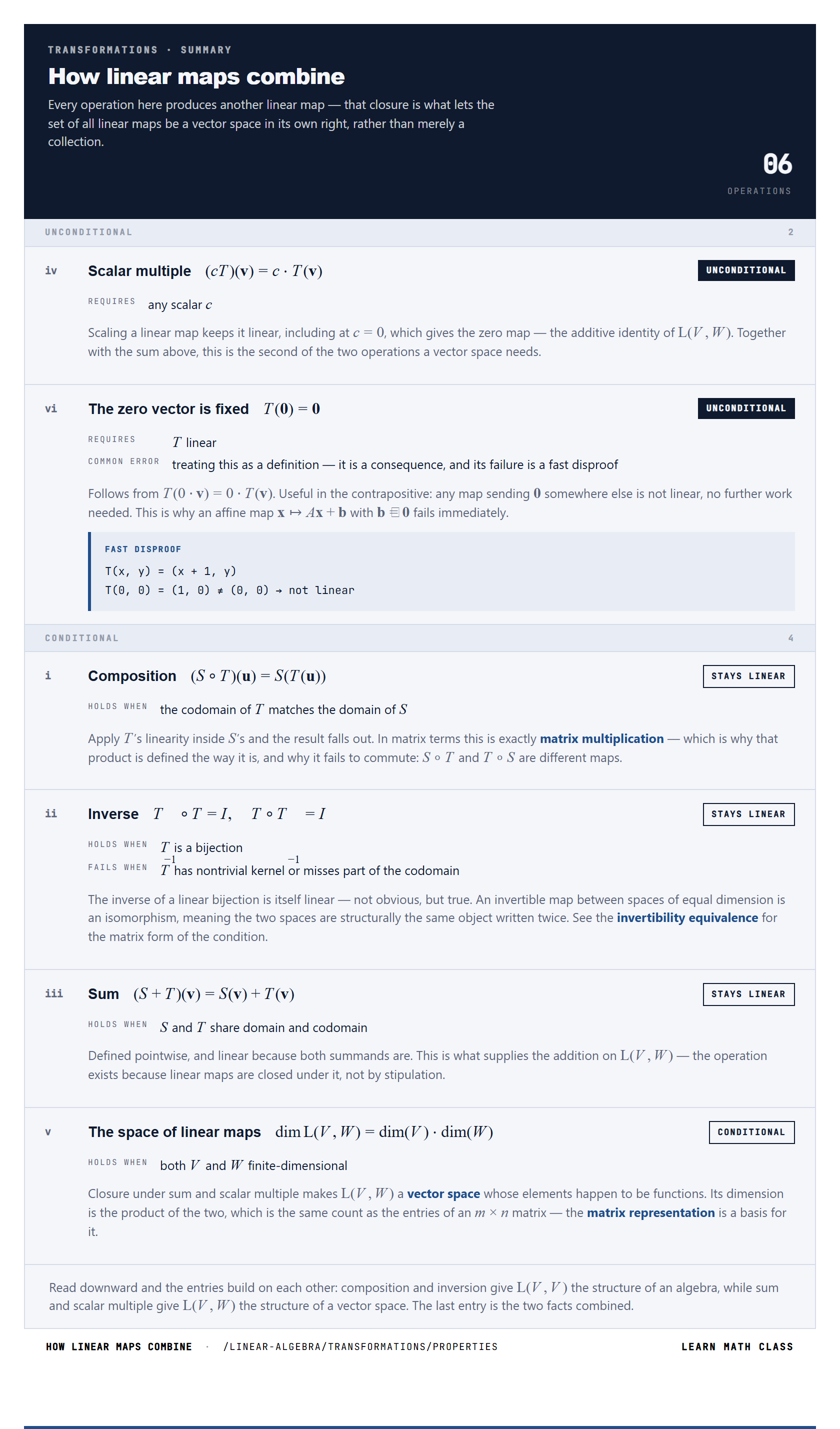
The four consequences-cluster sections above isolate distinct ways that linearity propagates through operations on the transformations themselves. The table below collects them in one place: composition produces another linear map, inversion preserves linearity, and the pointwise sum and scalar multiple of linear maps are themselves linear — giving the full set of all linear transformations from V to W the structure of a vector space in its own right.

Download

PNGRaster · 2×PDFPrint quality

Transformations · summary

How linear maps combine

Every operation here produces another linear map — that closure is what lets the set of all linear maps be a vector space in its own right, rather than merely a collection.

06operations

Unconditional2

iv

Scalar multiple§ 8

(cT)(\mathbf{v}) = c \cdot T(\mathbf{v})

Scaling a linear map keeps it linear, including at c = 0, which gives the zero map — the…

Unconditional

Requires: any scalar $c$

Scaling a linear map keeps it linear, including at $c = 0$ , which gives the zero map — the additive identity of $\mathcal{L}(V, W)$ . Together with the sum above, this is the second of the two operations a vector space needs.

vi

The zero vector is fixed§ 5

T(\mathbf{0}) = \mathbf{0}

Follows from T(0 · v) = 0 · T(v).

Unconditional

Requires: $T$ linear
Common error: treating this as a definition — it is a consequence, and its failure is a fast disproof

Follows from $T(0 \cdot \mathbf{v}) = 0 \cdot T(\mathbf{v})$ . Useful in the contrapositive: any map sending $\mathbf{0}$ somewhere else is not linear, no further work needed. This is why an affine map $\mathbf{x} \mapsto A\mathbf{x} + \mathbf{b}$ with $\mathbf{b} \neq \mathbf{0}$ fails immediately.

Fast disproofT(x, y) = (x + 1, y)
T(0, 0) = (1, 0) ≠ (0, 0) → not linear

Conditional4

i

Composition§ 6

(S \circ T)(\mathbf{u}) = S\bigl(T(\mathbf{u})\bigr)

Apply T’s linearity inside S’s and the result falls out.

Stays linear

Holds when: the codomain of $T$ matches the domain of $S$

Apply $T$ ’s linearity inside $S$ ’s and the result falls out. In matrix terms this is exactly matrix multiplication — which is why that product is defined the way it is, and why it fails to commute: $S \circ T$ and $T \circ S$ are different maps.

ii

Inverse§ 7

T^{-1} \circ T = I, \quad T \circ T^{-1} = I

The inverse of a linear bijection is itself linear — not obvious, but true.

Stays linear

Holds when: $T$ is a bijection
Fails when: $T$ has nontrivial kernel or misses part of the codomain

The inverse of a linear bijection is itself linear — not obvious, but true. An invertible map between spaces of equal dimension is an isomorphism, meaning the two spaces are structurally the same object written twice. See the invertibility equivalence for the matrix form of the condition.

iii

Sum§ 8

(S + T)(\mathbf{v}) = S(\mathbf{v}) + T(\mathbf{v})

Defined pointwise, and linear because both summands are.

Stays linear

Holds when: $S$ and $T$ share domain and codomain

Defined pointwise, and linear because both summands are. This is what supplies the addition on $\mathcal{L}(V, W)$ — the operation exists because linear maps are closed under it, not by stipulation.

v

The space of linear maps§ 8

\dim \mathcal{L}(V, W) = \dim(V) \cdot \dim(W)

Closure under sum and scalar multiple makes L(V, W) a vector space whose elements happen to be…

Conditional

Holds when: both $V$ and $W$ finite-dimensional

Closure under sum and scalar multiple makes $\mathcal{L}(V, W)$ a vector space whose elements happen to be functions. Its dimension is the product of the two, which is the same count as the entries of an $m \times n$ matrix — the matrix representation is a basis for it.

Unconditional

Conditional

Composition§ 6Stays linear

(S \circ T)(\mathbf{u}) = S\bigl(T(\mathbf{u})\bigr)

Holds when: the codomain of $T$ matches the domain of $S$

Apply

T

’s linearity inside

S

’s and the result falls out. In matrix terms this is exactly matrix multiplication — which is why that product is defined the way it is, and why it fails to commute:

S \circ T

and

T \circ S

are different maps.

Read the full section

Inverse§ 7Stays linear

T^{-1} \circ T = I, \quad T \circ T^{-1} = I

Holds when: $T$ is a bijection
Fails when: $T$ has nontrivial kernel or misses part of the codomain

The inverse of a linear bijection is itself linear — not obvious, but true. An invertible map between spaces of equal dimension is an isomorphism, meaning the two spaces are structurally the same object written twice. See the invertibility equivalence for the matrix form of the condition.

Read the full section

Sum§ 8Stays linear

(S + T)(\mathbf{v}) = S(\mathbf{v}) + T(\mathbf{v})

Holds when: $S$ and $T$ share domain and codomain

Defined pointwise, and linear because both summands are. This is what supplies the addition on

\mathcal{L}(V, W)

— the operation exists because linear maps are closed under it, not by stipulation.

Read the full section

Scalar multiple§ 8Unconditional

(cT)(\mathbf{v}) = c \cdot T(\mathbf{v})

Requires: any scalar $c$

Scaling a linear map keeps it linear, including at

c = 0

, which gives the zero map — the additive identity of

\mathcal{L}(V, W)

. Together with the sum above, this is the second of the two operations a vector space needs.

Read the full section

The space of linear maps§ 8Conditional

\dim \mathcal{L}(V, W) = \dim(V) \cdot \dim(W)

Holds when: both $V$ and $W$ finite-dimensional

Closure under sum and scalar multiple makes

\mathcal{L}(V, W)

a vector space whose elements happen to be functions. Its dimension is the product of the two, which is the same count as the entries of an

m \times n

matrix — the matrix representation is a basis for it.

Read the full section

The zero vector is fixed§ 5Unconditional

T(\mathbf{0}) = \mathbf{0}

Requires: $T$ linear
Common error: treating this as a definition — it is a consequence, and its failure is a fast disproof

Follows from

T(0 \cdot \mathbf{v}) = 0 \cdot T(\mathbf{v})

. Useful in the contrapositive: any map sending

\mathbf{0}

somewhere else is not linear, no further work needed. This is why an affine map

\mathbf{x} \mapsto A\mathbf{x} + \mathbf{b}

with

\mathbf{b} \neq \mathbf{0}

fails immediately.

Fast disproofT(x, y) = (x + 1, y)
T(0, 0) = (1, 0) ≠ (0, 0) → not linear

Read the full section

Read downward and the entries build on each other: composition and inversion give

\mathcal{L}(V,V)

the structure of an algebra, while sum and scalar multiple give

\mathcal{L}(V,W)

the structure of a vector space. The last entry is the two facts combined.

How linear maps combine·/linear-algebra/transformations/propertiesLearn Math Class

Linearity Properties FAQ

Does $T(\mathbf{0}) = \mathbf{0}$ prove that a map is linear?

+

No, the implication runs one way only. Every linear map sends zero to zero, so failing the test disproves linearity outright, but passing it proves nothing. The map

T(x) = x|x|

sends

0

to

0

and is not linear. Use it to rule maps out quickly, never to rule them in.Read more →

Is the single-line linearity condition shorthand for the two separate ones?

+

It is genuinely equivalent rather than an abbreviation. Setting

c = d = 1

recovers additivity and setting

\mathbf{v} = \mathbf{0}

recovers homogeneity, so the one line implies both and both imply it. Read it as a hypothesis to be tested about a particular

T

, not an identity to be simplified.Read more →

Is $\mathcal{L}(V, W)$ a set of matrices?

+

No, its elements are maps, and a matrix appears only after a basis has been chosen at each end. The space is itself a vector space, with dimension

\dim(V) \cdot \dim(W)

, which is exactly the number of entries a representing matrix would have. Its zero element is the map sending everything to

\mathbf{0}_W

.Read more →

Properties of Linear Transformation

What Linearity Gives You and How to Verify It

The Two Linearity Conditions

Linearity Notation

Linearity Notation

The One-Step Test

Proving Linearity

Worked Example

Disproving Linearity

Consequences of Linearity

Composition

Invertibility

Sums and Scalar Multiples of Transformations

Common Pitfalls

Summary: How Linear Maps Combine

How linear maps combine

Linearity Properties FAQ

Does $T(\mathbf{0}) = \mathbf{0}$ prove that a map is linear?

Is the single-line linearity condition shorthand for the two separate ones?

Is $\mathcal{L}(V, W)$ a set of matrices?

Properties of Linear Transformation

What Linearity Gives You and How to Verify It

The Two Linearity Conditions

Linearity Notation

Linearity Notation

The One-Step Test

Proving Linearity

Worked Example

Disproving Linearity

Consequences of Linearity

Composition

Invertibility

Sums and Scalar Multiples of Transformations

Common Pitfalls

Summary: How Linear Maps Combine

How linear maps combine

Linearity Properties FAQ

Does T(0)=0T(\mathbf{0}) = \mathbf{0}T(0)=0 prove that a map is linear?

Is the single-line linearity condition shorthand for the two separate ones?

Is L(V,W)\mathcal{L}(V, W)L(V,W) a set of matrices?

Does $T(\mathbf{0}) = \mathbf{0}$ prove that a map is linear?

Is $\mathcal{L}(V, W)$ a set of matrices?