Random Variables

Key Terms

From Outcomes to Numerical Values

What a Random Variable Is

Types of Random Variables

Random Variables and Probability Statements

Why Random Variables Matter

Common Examples of Random Variables

Random Variable Notation

What Comes Next

Random Variables at a Glance

Random Variables FAQ

Random Variables: Turning Outcomes into Numbers

Probability begins with events, but many real questions are numerical:
how many times something happens, how long it lasts, or how large a value turns out to be.

Random variables make this transition possible.
They connect random experiments to numbers, allowing probability to describe counts,
measurements, and quantities in a precise and consistent way.

Once randomness is expressed numerically, probability can move forward — toward
distributions, averages, variability, and comparison of outcomes.

Key Terms

Random Variable— a function

X: \Omega \to \mathbb{R}

Discrete Random Variable— a random variable with countable range

Continuous Random Variable— a random variable taking values in an interval

Function of a Random Variable— a new variable

Y = g(X)

Sample Space— the domain

\Omega

of any random variable

Probability Mass Function—

p_X(x) = P(X = x)

, distribution of a discrete variable

Probability Density Function—

f_X(x)

, distribution of a continuous variable

Cumulative Distribution Function—

F_X(x) = P(X \leq x)

See All Probability Definitions →

From Outcomes to Numerical Values

Random experiments produce outcomes, not numbers.
A coin toss results in heads or tails, a dice roll produces faces, and an experiment
ends in one of many possible outcomes.

Many probability questions, however, are not about the outcomes themselves but about
numerical results derived from them.
Counting successes, summing values, or recording measurements all require assigning
numbers to outcomes.

A random variable performs exactly this role: it assigns a numerical value to each
possible outcome of a random experiment, making quantitative probability analysis
possible.

What a Random Variable Is

A random variable is a mathematical construct that represents the numerical outcome of a random experiment or event. It acts as a function that assigns real numbers to each possible outcome of the experiment, with the understanding that multiple outcomes may result in the same value. The randomness associated with a random variable stems from the unpredictable nature of the underlying event, rather than the variable itself.

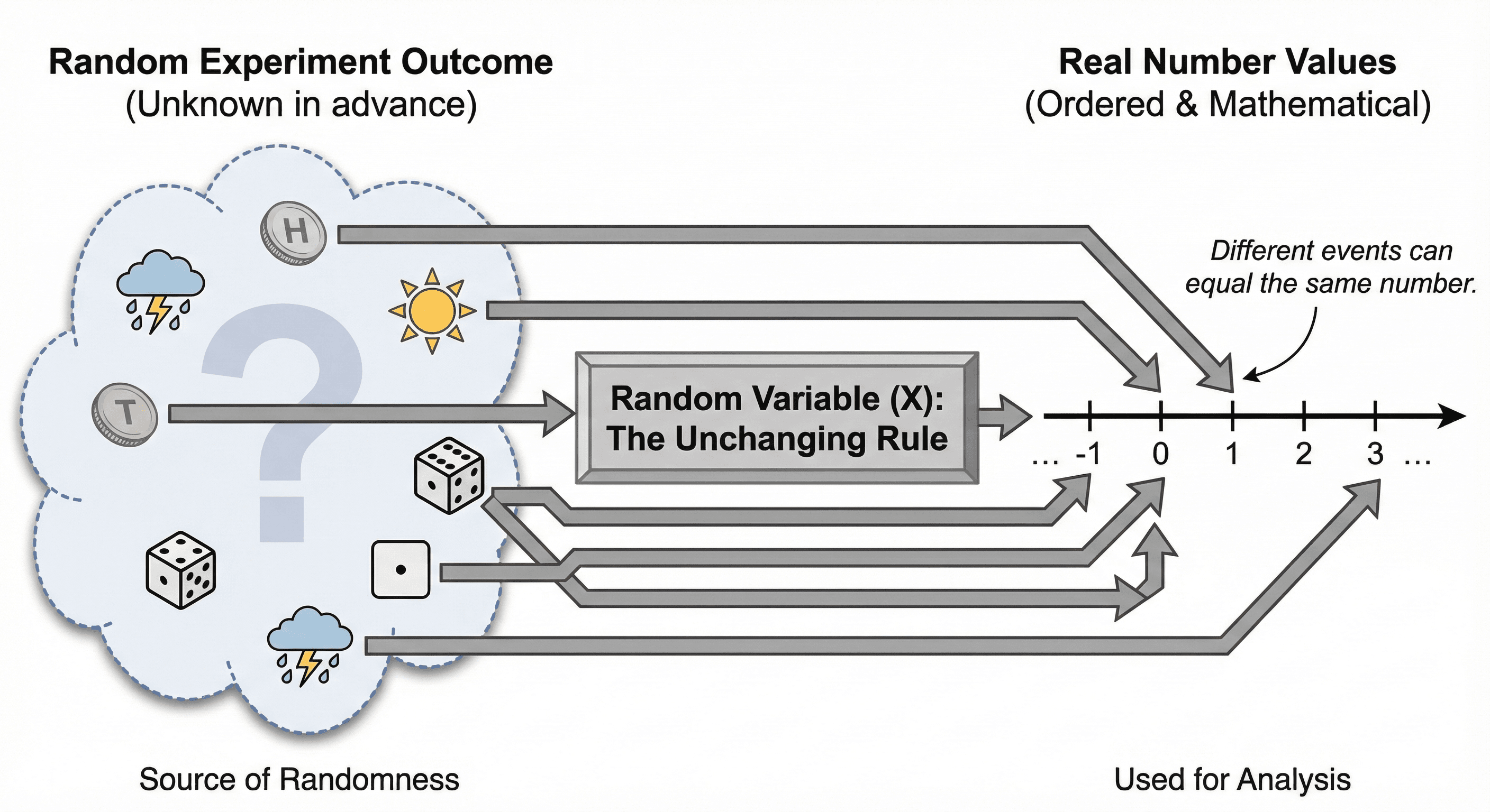
Random variables provide a means to quantify and manipulate probabilities using mathematical tools such as calculus. They offer a flexible and powerful framework for modeling various real-world phenomena that exhibit randomness. For example, consider rolling a six-sided die: the outcome of this event can be represented by a random variable X, which takes on values ranging from 1 to 6 with equal probability.

Random variables are essential in probability theory and statistics, as they allow for the development of probability distributions, such as the binomial distribution, normal distribution, and Poisson distribution. These distributions describe the likelihood of various outcomes occurring and provide important insights into the behavior of random events.

One can also define continuous random variables to represent outcomes that can take on an infinite number of values within a given range. For instance, the height of adult humans or the lifetime of a light bulb may be modeled as continuous random variables.

In summary, a random variable is a powerful mathematical tool for representing and analyzing the outcomes of random events using probabilistic methods. By assigning real numbers to each possible outcome of an experiment, we can study probability distributions, make predictions, and optimize decisions in various fields, including finance, engineering, economics, and science.

Types of Random Variables

Random variables are commonly classified according to the kinds of values they can take.

Discrete Random Variables

A discrete random variable takes isolated, countable values.
These values can be listed individually, even if the list is infinite.

Discrete random variables typically arise from counting processes, such as the number
of successes in repeated trials or the outcome of a dice roll.

Continuous Random Variables

A continuous random variable takes values from intervals of real numbers.
Its possible values form a continuum rather than separate points.

Continuous random variables usually arise from measurement, such as time, length,
weight, or temperature.

Attribute	Discrete random variable	Continuous random variable
Range	a countable set of isolated values	an interval (or union of intervals) of real numbers
Listability	values can be listed individually, even if infinitely many	values form a continuum and cannot be listed point by point
Typical source	counting processes (successes, occurrences, items)	measurement (time, length, weight, temperature)
Example ranges	{0, 1, 2, …}; {1, 2, 3, 4, 5, 6}	[0, ∞); [0, 1]; (−∞, ∞)
Probability function	probability mass function p_X(x) = P(X = x)	probability density function f_X(x)
Example variables	number of heads, face value of a die, indicator of an event	time until arrival, height, weight, temperature

Random Variables and Probability Statements

Once outcomes are represented numerically, probability statements can be written in
terms of random variables.

Instead of describing events directly, we describe conditions on numerical values,
such as a variable equaling a value or falling within an interval.
This allows probabilities to be written in forms like the probability that a random
variable takes a specific value or lies between two bounds.

Rewriting events in this way makes probability expressions easier to analyze and
prepares the ground for probability functions and distributions introduced later.

Why Random Variables Matter

Random variables are the link that allows probability to move beyond describing events
and toward analyzing quantities.

They make it possible to summarize randomness using numbers, compare outcomes across
experiments, and study patterns in uncertain situations.
Concepts such as averages, spread, dependence, and long-term behavior all rely on
random variables.

Without random variables, probability would remain purely event-based and could not
support distributions, expectation, variance, or any of the tools used in modern
probability and statistics.

Common Examples of Random Variables

Random variables appear naturally whenever outcomes are counted or measured.

A coin-toss experiment may define a random variable as the number of heads obtained.
Rolling dice can produce a random variable equal to the face value or the sum of
multiple rolls.
In measurement-based experiments, a random variable may represent time, distance,
weight, or temperature.

In many models, simple indicator variables are used, taking the value 1 when an event
occurs and 0 when it does not.

Random Variable Notation

Notation

Random Variable Notation

Three marks make a random variable usable: the signature that reveals it is a function, the braces that turn its values into events, and the tilde that names the distribution it follows. All of them are catalogued among the probability symbols.

The capital-versus-lowercase convention —

X

for the variable,

x

for a value it takes — is owned by the probability function, along with

P(\cdot)

p(x)

and

f(x)

; the sample space

\Omega

and its outcomes

\omega

by sample space notation.

X : \Omega \to \mathbb{R}

X maps the sample space to the real numbers

The signature exposes what a random variable really is — not a variable at all, but a function assigning a number to every outcome. The arrow signature is ordinary function notation, applied to the sample space as domain.

CasesWritten out,

X(\omega)

names the value at a particular outcome — the spelling that makes formulas like

E[X] = \sum X(\omega)P(\omega)

readable; everyday work suppresses the argument and writes just

X

Do not confuseAn unknown to solve for. Algebra's

x

waits for a value; a random variable already is the rule — there is nothing to solve, only outcomes to feed it.

\{X \le x\}

the event that X is at most x

Braces turn a condition on the variable into an event — a subset of the sample space, exactly the kind of object the probability operator

P(\cdot)

can measure. This is why

P(X \le x)

is well-formed: the inequality names a set, not a number.

CasesThe braces are routinely dropped inside

P

—

P(X \le x)

rather than

P(\{X \le x\})

— and the same shorthand covers

\{X = x\}

\{X > 3\}

\{a \le X \le b\}

; the cdf is built entirely from the

\le

form.

Do not confuseAn algebraic inequality to solve.

\{X \le x\}

is not a constraint on

x

— it collects the outcomes where the variable lands at or below

x

, which is a set, and the probability of that set is what follows.

X \sim \text{Bin}(n, p)

X is distributed as; X follows

The tilde declares which distribution governs a variable, with the parameters in parentheses —

X \sim \text{Bin}(n, p)

X \sim N(\mu, \sigma^2)

. One symbol replaces a paragraph: it fixes the whole probability function at once.

CasesParameter conventions vary by family and must be read from the source — the normal is written

N(\mu, \sigma^2)

with a variance in most texts but

N(\mu, \sigma)

with a standard deviation in some software; the distributions pages state each convention explicitly.

Do not confuseEquality or approximation. The tilde does not say

X

equals anything — it names a law, and elsewhere the same glyph means "approximately" or "asymptotically equal", which is why

X \sim N(0,1)

and

f(n) \sim g(n)

are unrelated statements.

All probability symbols →↑ Probability

What Comes Next

Once randomness is represented numerically, probability can be described using
functions that assign probabilities to values or intervals.

Random variables lead directly to probability distributions and to tools that summarize
and analyze their behavior, such as expectation and variance.
They also make it possible to study relationships between multiple quantities in joint
and conditional settings.

The next pages build on this idea by introducing probability distributions and the
functions used to describe them.

Random Variables at a Glance

The page has shown that random variables turn outcomes into numbers, that they come in discrete and continuous flavors, and that a small set of notational conventions makes probability statements precise and unambiguous. The table below collects these threads into a single reference card, with each row pairing an aspect of random variables with its formal statement and a concrete example or symbol illustrating it.

Aspect	Statement	Example or symbol
What a random variable is	a function X: Ω → ℝ that assigns a real number to each outcome of an experiment	rolling a die: X(face) = the face number
Where the randomness lies	in the underlying experiment; the variable itself is a fixed rule	the flip of a coin is random; labeling H = 1, T = 0 is fixed
Discrete type	range is a countable set of isolated values	X ∈ {1, 2, 3, 4, 5, 6}
Continuous type	range is an interval of real numbers	X ∈ [0, ∞) for time until an event
Notation for the rule	capital letter, referring to the entire assignment	X, Y, Z
Notation for a value	lowercase letter, referring to a specific result after the experiment	x, y, z — e.g. “X = 4” means the die landed on 4
Probability statements	events rewritten as conditions on the variable's value	P(X = x), P(X ≤ x), P(a ≤ X ≤ b)
Indicator variable	a special binary random variable marking whether an event occurs	1_A = 1 if A occurs, 0 otherwise
What random variables enable	a numerical framework for analyzing randomness	distributions, expectation, variance, comparison across experiments

Random Variables FAQ

Why is a random variable called a variable if it's a function?

The name is historical and misleading. The signature X : Ω → ℝ says what it really is: a function assigning a number to every outcome. Written in full, X(ω) is the value at a particular outcome; everyday work drops the argument and writes just X. It is not an unknown waiting to be solved for — the rule already exists, and outcomes get fed into it.Read more →

What does P(X ≤ x) actually mean?

It is the probability of a set. The condition X ≤ x collects every outcome where the variable lands at or below x, and that collection is an event — a subset of the sample space, which is the only kind of thing P can measure. Written strictly it is P({X ≤ x}); the braces are dropped by convention. It is not an inequality to solve.Read more →

What does the ~ symbol mean in X ~ N(μ, σ²)?

It reads “is distributed as” — the variable follows that distribution, with the parameters in parentheses. One symbol replaces a paragraph, fixing the entire probability function at once. It does not assert equality or approximation: X ~ N(0,1) names a law, whereas the same glyph in f(n) ~ g(n) means asymptotically equal.Read more →

What are the parameters in a distribution declaration?

Whatever the family specifies, in the order that family fixes — and the notation does not say what they mean. Bin(n, p) takes trials then success probability; Exp(λ) takes a rate; N(μ, σ²) takes a centre then a spread. The conventions vary by family and by author, so the distributions pages state each one explicitly.Read more →